What if adversarial defenses just need more JPEG?

When machine learning models get deployed into production, the people who trained the model lose some amount of control over inputs that go into the model. There is a large body of literature on all the natural ways in which the data a model sees at inference time might be different than the data the model saw during training. For example, if your model is trained to identify photographs of cell phones from the early 2000s like this one:

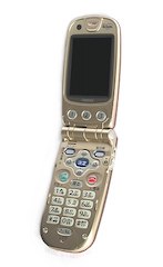
_{By Qurren - Own work, CC BY-SA 3.0, https://commons.wikimedia.org/w/index.php?curid=750637}

It is going to fail to identify photographs of cell phones from the late 2000s, like this one:

_{By Justin14 - Own work, CC BY-SA 3.0, https://commons.wikimedia.org/w/index.php?curid=25401575}

Your model is effectively frozen in time to the years covered by the data it was trained on, but the world moves on, and people mostly don't use flip phones anymore. This change in the visual aspects of what constitutes a "cell phone" is a kind of distribution shift, and is a naturally occurring process.

The most common strategy to make models robust in the face of unknown inputs like newer kinds of cell phones is frequent re-training on new data, but there is a kind of unusual input where frequent retraining will not help. These are unusual inputs that are made by someone to look unusual on purpose.

The phenomenon of creating inputs that cause machine learning models to malfunction has been known for some time, but gained prominence in the era of deep neural networks (DNNs) because of how much easier it is to create these adversarial examples for neural network architectures. A new exploit -- or an improvement on a previously known exploit -- gets published on arxiv about every other day, so the threat of adversarial attacks on production systems has been growing quickly.

In our last blog post we saw that one strategy for handling adversarial attacks against your model was to place adversarial attacks in the data, and then use that for training (see Poisoning your model on purpose). This works well if you know (or can guess) in advance how your model will be attacked, and comes with some guarantees about robustness, but has the tradeoffs of making model training take longer, and, sometimes, reducing accuracy on clean (e.g. non-attacked) data.

Another way to think about this problem is in terms of mutating adversarial inputs back to regular inputs, perhaps by having some understanding of the differences between adversarial noise and run of the mill data collection noise. In the case of images specifically, the classic adversarial attacks tend to add low magnitude, high frequency noise, in a way that humans can't detect:

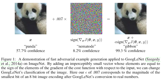
At the level of the actual pixel magnitudes though, this makes adversarial inputs look quite a bit different than clean samples. An obvious first thought is that adding some gaussian blurring, or removing all of the high spatial frequency components from the image, would remove the adversarial attack too.

This is true, but a lot of what the model is paying attention to are those high frequency details, so this has the potential downside of harming model accuracy on clean inputs. What we want then is some sort of image compression algorithm that only keeps the useful details, and gets rid of the useless details, in the input. The question then is how to tell the difference between the useful signals and the useless signals.

A data-driven way to approach this is to use a kind of model called an autoencoder. This is a generic name for a model that takes an input and tries to generate an output that is very similar to the input. Now, obviously if you have a large enough model, it will just copy the pixel values directly from the input to the output, so typically autoencoders are much smaller than their inputs. This means you have a model that learns from the data how best to compress the information on the way in, and then reconstruct an image from that compressed representation on the way back out.

This is the approach taken by Meng and Chen in their 2017 paper, "MagNet: a two-pronged defense against adversarial examples".¹ They train an autoencoder on both MNIST (images of hand-written digits) and CIFAR-10 (low-resolution images of objects), and use them to clean up adversarial inputs generated by the fast gradient sign method (FGSM), DeepFool, and Carlini-Wagner.

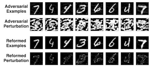
Here's an example of what that looks like for MNIST. The first row in this figure shows digits with adversarial noise added to them. The second row is just the additive noise from the Carlini-Wagner attack, exaggerated to make it easier to see. The third row is the same set of digits, but after they have been passed through the MNIST autoencoder, and the fourth row shows the remaining adversarial noise that is left over after cleaning. You'll notice that, after cleaning, the noise is broadly confined to the edges of the actual digit, and the pixel changes in the rest of the square are mostly gone.

How much does this help classification accuracy against adversarially generated inputs? Not as much as you might hope. The blue line in the following figure shows the accuracy of the classifier after using the autoencoder (they call this their "reformer") on the y-axis, as a function of how different the adversarial input is from a normal image of a handwritten digit on the x-axis. For non-obvious amounts of additive noise the reformer defense keeps accuracy almost at 100%, which is great! But for larger amounts of noise, the autoencoder isn't much better than having no defense at all.

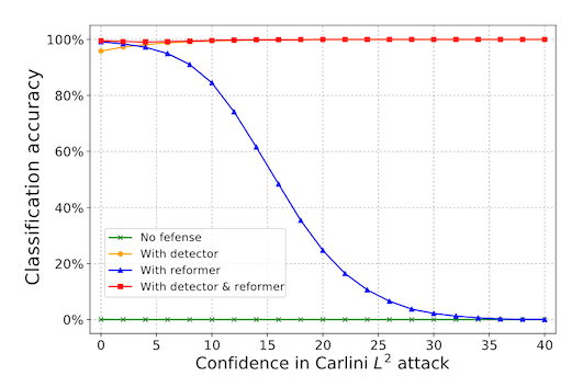
"Non-obvious" and "obvious" amounts of noise are relative here, because that x-axis is really showing how confident a different model is that a particular input has been attacked. That's a topic for the next blog post, but we'll just say for now that stronger, more obvious attacks should be easier to detect, so our approximate description of that plot is technically wrong but directionally correct.

Also, to be fair to the authors, their actual defense includes a second component, and combined together gives much better accuracy against attacked inputs -- say, 80% on average for CIFAR-10. Again, we'll talk about this more in the next blog post!

The disadvantages of this method are two. First, the limited ability of the autoencoder to strip the adversarial attack off of the image and recover good test accuracy on its own. And the second is that now you have to train, track, and deploy a second model along with the first one. And as the famous saying goes, if you solve a problem with a machine learning model, now you have two problems. If you solve a problem with two machine learning models...

So as a reminder, what we want here is something that preserves the useful high frequency information in an image, but strips out the useless stuff. It turns out, there is an out-of-the-box algorithm for doing this; it's been around for 30 years, and its already available on every operating system

You probably guessed it from the title. JPEG!

The idea behind JPEG is to compress an image in a way that keeps it looking similar to the human visual system by discarding information that humans pay less attention to. So, for example, it is more likely to keep high frequency information about luminance than about color, because humans pay more attention to shapes when identifying objects in a visual scene. It keeps more of the low-frequency luminance information than the high-frequency luminances, because humans pay more attention to shape than to textures.

We saw earlier (see Natural adversarial examples) that models have the opposite priority, and pay a lot of attention to colors and textures. Here is an example of what JPEG compression looks like (to you, a human, I presume):

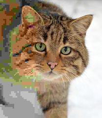
_{By Felis_silvestris_silvestris.jpg: Michael Gäblerderivative work: AzaToth - Felis_silvestris_silvestris.jpg, CC BY 3.0, https://commons.wikimedia.org/w/index.php?curid=16857750}

In 2017, Das et al. investigated the use of JPEG compression to remove adversarial noise, and help computer vision models recover good test accuracy on adversarially perturbed images.² They train image classification models on two tasks: CIFAR-10, which we saw before, and GTSRB, a road sign classification dataset. In each case, they create adversarial attacks on the test set (FGSM and DeepFool), then compress them with JPEG before giving them to the model for inference.

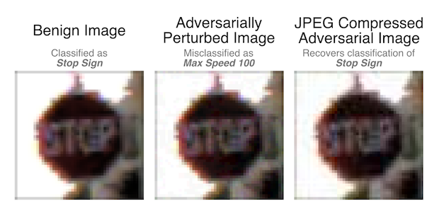
And it works pretty well! In the plot below, the solid lines are the attack success for JPEG only, so lower is better. Using a JPEG quality of 75% during compression works very well on DeepFool, but a little less well on FGSM.

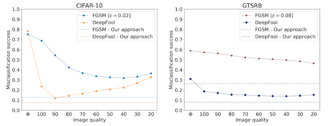
A potential problem with this approach is that we have now introduced our own form of distribution shift! These models were trained on lossless images, and we're giving them compressed ones, which is likely to hurt model accuracy on both clean and perturbed samples.

The solution? It needs more JPEG!

In the next experiment, the authors train their image classification models on datasets where the training data has also been compressed with JPEG, and then use the same amount of JPEG compression on adversarially perturbed examples. And the results are looking a lot better! Before our accuracy against attacked images was maybe 40% to 60%, but by training on these JPEG images the accuracy goes from 60% to 90% (again, depending on the dataset and attack method). In the plot below, the y-axis is model accuracy, so higher is better.

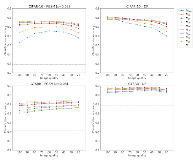
And there you have it -- a surprisingly cheap, widespread, and effective way to defend computer vision models against adversarial inputs. Assuming, of course, that you can train your own computer vision model.

 

Is this interesting?

Get an email about the next blog post